
What are some of the fundamental principles that govern the reactivity of molecules? What makes a molecule a good nucleophile or a strong electrophile? How can we predict which position of an aromatic ring undergoes electrophilic or nucleophilic substitutions? The simple understanding that a nucleophile is electron-rich molecule that attacks sites with low electron density, and that electrophile is electron-poor molecule that will attack a position of large electron density allows to understand many organic reaction.
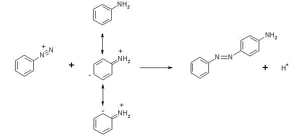
For example, consider a diazo coupling reaction in which benzenediazonium chloride reacts with aniline. One can deduce from the positive charge that the diazonium group is very electron-poor, and thus acts as a good electrophile. Aniline acts as a nucleophile but what is the nucleophilic site? Recall that in aniline, the lone pair of the amino group is delocalized. Consideration of possible resonance contributors to the conclusion that the ortho and para-positions in aniline are nucleophilic. The ortho position is sterically hindered, and one could correctly predict that the azo compound forms when the electrophile attacks the para position of aniline.
In other situations, this simple understanding is insufficient. For example, how can we rationalize the observed preference of nitration of the 1-position in naphthalene by nitric acid if the total π electron densities in the 1 and 2 position are expected to be the same? Recall that in the nitration reaction, nitronium ion (NO2+) acts as an electrophile, and naphthalene behaves as a nucleophile. But which position in naphthalene is more nucleophilic? In principle, the answer can be reached by considering the structures and energies of the two transition states leading to the two products but this approach is often impractical.
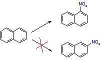
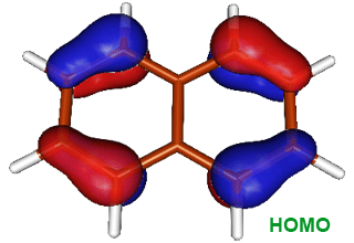 A powerful practical model for describing chemical reactivity is the frontier molecular orbital (FMO) theory, developed by Kenichi Fukui in 1950's. The important aspect of the frontier electron theory is the focus on the highest occupied and lowest unoccupied molecular orbitals (HOMO and LUMO). For example, instead of thinking about the total electron density in a nucleophile, we should think about the localization of the HOMO orbital because electrons from this orbital are most free to participate in the reaction. The image on the right shows the distribution of HOMO in naphthalene; we can see that the frontier electron density is highest at the position 1. Thus, the electrophile reacts with position 1 of naphthalene.
Similarly, the frontier orbital theory predicts that a site where the lowest unoccupied orbital is localized, is a good electrophilic site. The FMO theory was initially used for explaining the electrophilic substitution in naphthalene but it became gradually clear that the scope of this theory is much broader. For example, the concept of frontier orbital symmetries was successfully used to rationalize the outcomes of cycloaddition reactions and other pericyclic reactions. Frontier molecular orbital models for some organic compounds are available here.
You can read more about the frontier orbital theory from Kenichi Fukui Nobel Prize lecture.
Standard quantum chemistry calculations yield delocalized molecular orbital. In Gaussian, keyword Pop requests printout of molecular orbitals. Alternatively, keywords GFINPUT, IOP(6/7)=3 can be used to ccreate output that can be visualized with MOLDEN. Your directory on the workstation contains a file naphthalene_TZ_MPD.out that contains MO information on naphthalene. You do not need to repeat this calculation because it will be time consuming. Also notice that this calculation included some treatment of electron correlation by invoking the MP2 keyword; the result of this is that many MO orbitals will have fractional populations.
You can read more about the frontier orbital theory from Kenichi Fukui Nobel Prize lecture.
The shape of a molecule is determined by the electron density of the molecule and this electron density depends on the atomic composition of the molecule. One way to determine molecular shape is to calculate electron density and display the region where electron density is larger than some cut-off value as a three-dimensional surface. Such calculations necessitate quantum chemical approach and are possible with not too large molecules. For larger molecules, Connolly surfaces and solvent-accessible surfaces can be calculated rapidly based on empirical van der Waals radii of atoms.

Electrostatic potential surfaces are valuable in computer-aided drug design because they help in optimization of electrostatic interactions between the protein and the ligand. These surfaces can be used to compare different inhibitors with substrates or transition states of the reaction. Electrostatic potential surfaces can be either displayed as isocontour surfaces or mapped onto the molecular electron density. The latter are more widely used because they retain the sense of underlying chemical structure better than isocontour plots.
 This tutorial illustrates how to use quantum chemistry calculations to generate and display molecular electron density surfaces and map electrostatic potential values to the surface. You will compare two conformers of oxamic acid. Oxamate, anion of oxamic acid is a powerful inhibitor for Plasmodium falciparum lactate dehydrogenase and thus may serve as a fragment or lead in developing novel anti-malaria drugs. The molecule has two low energy conformers that differ in the dihedral angle about the central C-C bond. These conformers are shown in the image on the right.
Your task is to calculate and display electrostatic potential of cis and trans oxamic acid. Molecular surfaces should be calculated based on optimized molecular geometries. While molecular mechanics force fields can be used to generate reasonable initial geometries, it is considered a good practice to optimize molecular geometries with quantum mechanical methods prior generation of electron molecular electrostatic potential surfaces. In this tutorial you start with previously optimized structures of cis and trans oxamic acid because optimization jobs can be time-consuming. The quantum chemistry program Gaussian was used to perform geometry optimization for the two conformers. The calculation was performed at the Moller-Plesset second order perturbation theory level with a moderate-sized basis set to describe molecular orbitals. Specifically, a 6-311+G(d,p) basis set was used which allows for some polarization of electron density on both heavy atoms and hydrogens. In computational jargon, the molecule was optimized at the MP2/6-311+G** level. The comparison of relative energies of the two conformers suggests that s-trans conformer is more stable by 1.68 kcal/mol. You can use MOLDEN to launch quantum mechanical geometry optimizations but keep in mind that optimizing a larger molecule using accurate QM methods can be very time-consuming.
You will be performing these calculations on a remote workstation. The files that you need to start the calculation are on your SGI directory, though. You can transfer files between computers using File Transfer Protocol, or FTP. You can access your files from the workstation by opening an ftp connection to the SGI file server (the address will be given in the class). After opening the FTP connection, navigate to your directory on the SGI file server by typing cd PERM where PERM is your perm number and hit enter. Then transfer the two input files to the workstation by typing get oxamic_ac_trs.mol2 and get oxamic_ac_cis.mol2. Exit the ftp program by typing bye. Verify that the input files are in your directory on the workstation.